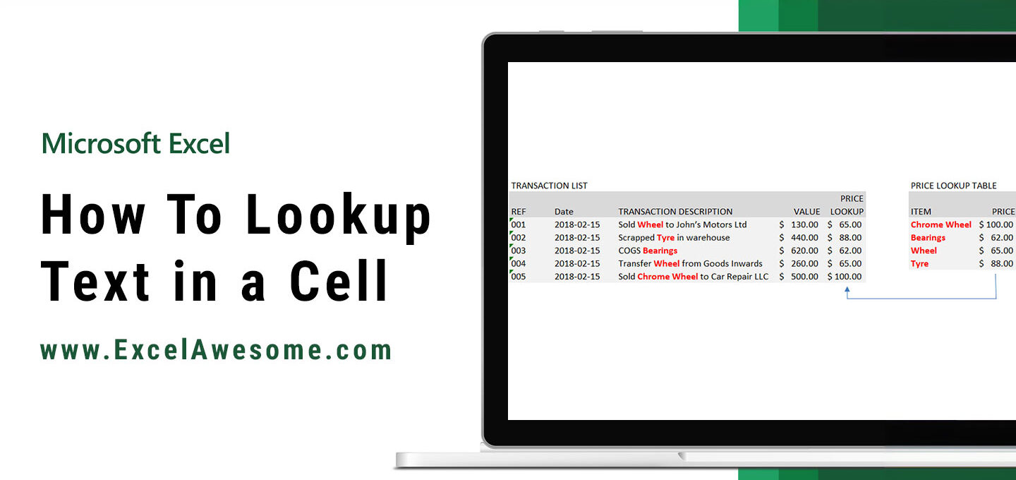
In Excel you may need to lookup just part of the text in a cell. For example, if you have a cell that contains a transaction description and within that description there is a product name.

You want to lookup the price of that product from a table. Let’s look at three possibilities:
- When the product name is just randomly placed within the lookup text: “Sold WHEEL to John’s Motors Ltd”
- As 1. above but there are always defined characters before and after the product name: “Sold –WHEEL– to John’s Motors Ltd”
- The product name is always in the same part of the string: “AA2 WHL Sold – JM1″
Obviously the third possibility in the list is the easiest to solve in Excel so lets begin there.
Lookup Part of Text in Cell: Consistent Start and End Points
The VLOOKUP (or HLOOKUP) function has the following arguments: LOOKUP VALUE, TABLE, COLUMNS INDEX NUMBER, EXACT/NON-EXACT MATCH. As the LOOKUP VALUE is only part of the cell, we need to consider how we can extract the text we want from the cell.
Check FIG(a1) for the LOOKUP VALUE sources and TABLE ARRAY.
Find the LOOKUP VALUE Part of the Cell
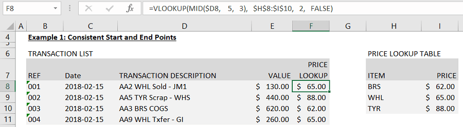
Since in this case the start point in each source cell is consistently character 5 and the length of the LOOKUP VALUE will always be 3 characters (such as “WHL” in cell D8), we can use the MID function to extract the LOOKUP VALUE. The MID function just needs the TEXT, START CHARACTER NUMBER and NUMBER OF CHARACTERS.
In our example lets start by inputting the MID function in cell F8. You can see the result in FIG(a2).
The result of this we now just need to use in our VLOOKUP formula. The LOOKUP TABLE being in range $H$8:$I$10, COLUMN INDEX NUMBER is 2 (the second column in the table) and in this case we only want to return exact matches so the final argument will be ‘FALSE’.
Finalize the Formula to Lookup Part of the Cell
Putting that formula together in our cell F8 is:
=VLOOKUP(MID($D8, 5, 3), $H$8:$I$10, 2, FALSE)
Copying down that formula next to our transactions completes the lookup of prices FIG(a3).
Moving on to our next scenario.
Lookup Part of Text: Using a Consistent Character as Separator
In this case we will use the separator ‘-‘ to define the start and end of the LOOKUP VALUES in the source cells. This method works as long as the separator character is only used to identify the Product Name. If appears elsewhere in the text then you can proceed to scenario 3 which can handle the LOOKUP VALUE anywhere in the cell.
Use the Dashes to Separate the LOOKUP VALUE
You can see in FIG(b1) that if we find the dashes ‘-‘ we will be able to extract the needed text using the MID function. To do this we will need to know the starting character for “Wheel” and the number of characters in “Wheel”. We will use the FIND function to identify the placement of our separators and do these calculations.
FIND first separator
In FIG(b2) you can see the make up of the FIND function to locate the start of “Wheel”. The FIND function has the following arguments: FIND TEXT, WITHIN TEXT and an optional CHARACTER START NUMBER. This third optional argument is useful when you are looking for the second or subsequent separator. We will use it later but for now we can ignore it.
So putting our FIND function in cell F17. [FIG(b2)] you can see it has returned the placement of the of the first dash.
=FIND(“-“, $D17)
FIND second separator
Now, lets find the second separator so we can find the end of our LOOKUP VALUE. We are going to do this by doing another FIND formula. This time though we will need to use the START NUMBER to make sure we skip past the separator we’ve already discovered.
In FIG(b3) you can see the first two arguments of the second FIND are exactly the same. But to skip over the first separator we need to get the number for this from cell F17 (+1 to jump past it).
=FIND(“-“, $D17, F17+1)
Use MID Function to Get the LOOKUP VALUE
Now we have those results we can put together a MID function (as used in the first scenario).
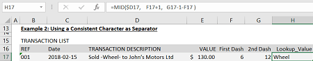
FIG(b4). The first argument of the MID function is just our transaction description. Second is the start point which is our first FIND function. Next we need the number of characters to extract. We can calculate this as our second FIND result less the first. You can see we have extracted the LOOKUP VALUE.
=MID($D17, F17+1, G17-1-F17)
Before going on to the last step lets combine our functions. You can do this by editing the cell with the first FIND and copying everything after the “=”. Leave this cell then edit our MID function in cell …. highlight the reference to cell …. and paste. Repeat this for the second FIND function. Great, that’s our MID function complete.
You should end up with this:
=MID($D17, FIND(“-“, $D17)+1, FIND(“-“, $D17,FIND(“-“,$D17)+1) -1 -FIND(“-“, $D17))
VLOOKUP part of text
Finally we can do our VLOOKUP using this MID function as the LOOKUP VALUE. In FIG(b6) you can see we’ve referenced this cell, input our table, selected the second column and indicated we want exact match (FALSE).
=VLOOKUP(F17, $J$17:$K$19, 2, FALSE)
We will just replace the reference to cell F17 with the formula in that cell. Copy that down and we’re done FIG(b7).
=VLOOKUP(MID($D17, FIND(“-“, $D17)+1, FIND(“-“, $D17,FIND(“-“,$D17)+1) -1 -FIND(“-“, $D17)), $J$17:$K$19, 2, FALSE)
There are a few steps there but hopefully the logic makes sense. Now lets move on to the final scenario where you can lookup pretty much any of the possible Product Names wherever they appear in our source text.
Lookup Part of Text: Randomly Placed Text in Cell
In order to lookup part of text in a cell that is randomly placed; we are going to need something other than the VLOOKUP function. Instead we are going to create a fairly complicated ARRAY FORMULA that uses INDEX, MATCH, ISERROR and FIND. If any of these functions are unfamiliar, don’t worry. Just follow it through. Once you’ve built the array formula hopefully you can understand the logic in those functions.
The Logic In This Solution
Lets consider the logic of this approach to look up part of the cell. We are going to use what I’ll call a reverse lookup. I.e. we’re going to try each of the items in column H (the first column of our lookup table) to see if the text in those cells is anywhere in our source cell (the descriptions in column D). Once we’ve found one that matches, we’ll look down the corresponding data in column I and get the result.
Ok, lets begin by seeing if we can find an item in column H that is in our lookup source cells.
ARRAY Formulas
An ARRAY formula allows us to use an array of values (compared with a standard equivalent formula where we’d just be able to use a single value).
You may be aware that the FIND function returns an error if it can’t locate the searched text. E.g. =FIND(“C”, “ABD”) returns an error.
So as part of an ARRAY formula, =FIND({“A”,”B”,”C”,”D”}, “SAMPLE TEXT”) would return {2,ERROR,ERROR,ERROR}.
Applying that to our data would result be: =FIND({“Chrome Wheel”,”Bearings”,”Wheel”,”Tyre”}, “Sold Wheel to John’s Motors Ltd”) and return {ERROR,ERROR,6,ERROR}
Hopefully you can see this may be useful. If we can identify where the first non-error occurs we can find the position in the table for our result.
MATCH Function In ARRAY FORMULA
To find the non-error we can use MATCH function to look through the results of the FIND array.
Before we do that lets use the ISERROR function to convert {ERROR,ERROR,6,ERROR} to {TRUE,TRUE,FALSE,TRUE}.
Now instead of numbers we have FALSE to look for.
The FALSE results are the nuggets we’re looking for.
To find the placement of the FALSE we can use the MATCH function. So “=MATCH(FALSE, {TRUE,TRUE,FALSE,TRUE}, 0)” in an ARRAY formula is going to return 3.
Lets try inputting the ARRAY FORMULA so far to make sure it is working as expected. See FIG(c1) for the formula.
{=MATCH(FALSE, ISERROR(SEARCH($H$31:$H$34, $D31)), 0)}
To enter an ARRAY formula, press SHIFT+CTRL+ENTER (rather than just ENTER). This tells Excel you want an array formula. You don’t type the leading and ending {}. Hitting SHIFT+CTRL+ENTER will put these in. Make sure you check these are shown once you’ve done the SHIFT+CTRL+ENTER.
You can see this is returning 3 which is the correct row in our table for “Wheel”.
Complete the Lookup with INDEX Function
We’re almost done with the tutorial. All we need to do now is use this result in an INDEX function.
If you’re not familiar with the INDEX function the arguments are: ARRAY, ROW NUMBER, and optional COLUMN number. We can complete this with one column so the final argument won’t be needed for this example.
So our INDEX function looks at the lookup table and identify the cell you want from the table by identifying which row to select from it.
Putting this altogether you can see the result in FIG(c2). So we’re looking down our table in column I by the number of rows identified by the MATCH function.
{=INDEX($I$31:$I$34, MATCH(FALSE, ISERROR(SEARCH($H$31:$H$34, $D31)), 0))}
We can copy this down and we have results for all our lookups.
What To Watch Out For
- The FIND function is case sensitive. To remove this sensitivity, you can either keep the data in column H in upper case and amend the formula to: INDEX($I$31:$I$34, MATCH(FALSE, ISERROR(FIND($H$31:$H$34, UPPER($D31))), 0)). Fig(c3). Or you can replace FIND with SEARCH. The SEARCH function is not case sensitive.
- You need to think about the order of your data in the lookup table. As Excel is going to run down the data in column H it will find the first match. A cell with the words “….CHROME WHEEL…” could match to both “WHEEL” and “CHROME WHEEL”. So in this case you’d want to ensure “CHROME WHEEL” was above “WHEEL” in your table. You may resolve this problem by sorting your list by length of “Product Name”.
Hopefully you find this functionality useful. If you have any questions or comments please post them below.
You can also learn how to create a hyperlink to VLOOKUP or SUMIF results.
And if you’re looking to include wildcards in the ‘lookup what’ then check out these wildcard examples.
Amazing resource. Thank you.