You may want to find and highlight all blank cells in a range or sheet within your Excel® file.
You can use conditional formatting to highlight if a cell is blank. And you can also use conditional formatting to highlight any of these cell attributes:
- Is text
- Is a formula
- Is a constant
- Is an error
- The number of characters
- Is protected
If you only need to do a one-off test for blanks or the other attributes above within your range then skip down to ‘One-off cell attribute tests’. This will be quicker than adding conditional formats for this type of query.
If you’re new to using formulas with Conditional Formatting then lets cover that first.
Conditional Formatting by Formula Result
1. Highlight the range where you want conditional formats (highlight from the top-left to the bottom-right of range)
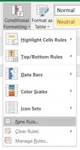
2. From the HOME RIBBON choose CONDITIONAL FORMATTING then click NEW RULE…
3. Click on ‘Use a formula to determine which cells to format’
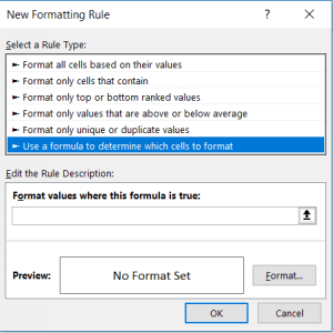
4. Put our formula in the ‘Format values where this formula is true:’
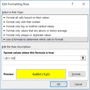
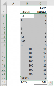
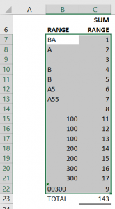
In this case lets test for any value greater than 100.
This formula here is similar to the first part of an IF function in Excel®. I.e. it is a formula that returns either TRUE or FALSE.
So we are going to enter the following formula in the field (where B7 is the top left cell in our range):
=B7>100 [include the ‘=’ at the start of the formula]
Excel® checks each cell relative to our starting position. So this test is for cell B7, In C7 Excel® will automatically test C7>100 and so on.
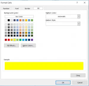
Now click on the Format… button and FILL with YELLOW.
Click OK three times to accept these changes.
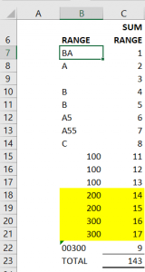
5. The result can be seen here
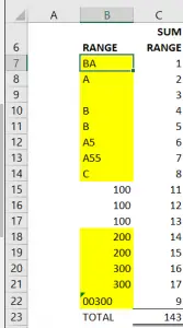
This result is probably not quite what we want. You can see the text and blank cells have been colored yellow as well as the values over 100.
6. Make changes to use COUNTIF function in test
Lets make changes to the formula trying an alternative method to identify the values over 100.
Highlight the range from B7 down to C22 again.
Then from the HOME RIBBON click CONDITIONAL FORMATTING and MANAGE RULES. Then click our rule and ‘EDIT RULE’.
We’re going to change the formula to the following (again this assumes we highlighted the cells beginning in cell B7 down to C22):
=COUNTIF(B7,“>100”)>0
The logic is to use the COUNTIF function to make sure that the single cell range has a value greater than 100. Again just focus on having this formula correct for the top-left cell and Excel® will take care of the other cells in the range.
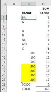
This result is now what we’re expecting.
That said, depending on the result we want, it may be better to color the entire row of data yellow. To do this we can repeat the EDIT RULE process and make a small edit to the formula.
7. Color entire row of data using CONDITIONAL FORMAT
If we consider how Excel® is applying our formula to each cell in the range then it should be apparent that we want to amend the color of cell C7 based on the test of cell B7. I.e. if B7 is greater than 100 then color C7 yellow. As with relative/absolute references in Excel® we can do this by locking the column address with the ‘$’ dollar sign.
=COUNTIF($B7,“>100”)>0
This simple change results in the following conditional format result:
Now we have covered the basics of using formulas in CONDITIONAL FORMATS lets look at how we can color blanks.
Conditional Formatting if Cell is BLANK
We’ll continue working with the same table as above. The process is going to be the same but we will use a different function in our formula.
The simplest solution is to use the COUNTIF function again.
=COUNTIF($B7,“”)
We can try this after editing our conditional format formula.
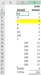
You can see this works as expected. If you clear out some of the other cells in colulmn B you will see they also turn yellow as expected.
Limitations of this method
The COUNTIF function will include all cells that appear to be blank.
There could potentially be a formula in cell B9 above that is returning “” [such as ‘=IF( C9=4, “A”, “”].
If you don’t want to highlight cells like this then we need an alternative function.
In fact there are 2 alternatives we could use.
=ISBLANK($B7)
=CELL(“type”,$B7)=”b”
The ISBLANK function is a simple test that exists in Excel® to return TRUE or FALSE. TRUE is only returned if there is no text, formula or constant in the cell.
However it is worth understanding the CELL function as this can be useful for applying conditional formatting to highlight cells with other attributes.
The CELL function has two arguments: INFO_TYPE and REFERENCE. You can select INFO_TYPE from a list of available options when you start typing the formula. INFO_TYPE is a series of attributes provided by Excel®. We need “type” for our formula. This identifies the type of contents in the reference cell.
The function will return either “b” for blank, “l” for label (text) or “v” for everything else.
Lets move on to look at conditionally formatting for other attributes:
Conditionally Formatting if Cell is Not Blank
This one is easy based on the ‘conditionally formatting if cell is BLANK’ example above.
All we need to do is replace our previous CELL function with:
=CELL(“type”,$B7)<>”b”
The change of ‘=’ to ‘<>’ is all that is needed.
Conditionally Formatting if Another Cell is Blank
It may be beneficial to use a cell at the top of a form to indicate if a cell that requires user input has been completed.
For example we may want to apply the conditional formatting to cell P1 to indicate that cell F23 is blank.
To do this we would select cell P1. Then follow the steps to create a conditional format condition.
The formula in the conditional format would be:
=CELL(“type”,$F$23)=”b”
Conditionally Formatting if Cell Contains Text
This is another condition the CELL function with “type” can resolve.
If we go back to the table in our earlier example. It is simply a case of again highlighting cells top-left to bottom-right cells B7:C22.
Edit the conditional formatting rule and change the formula to:
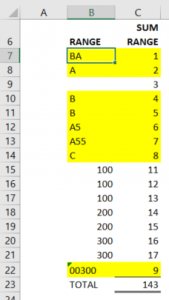
=CELL(“type”,$B7)=”l”
“l” represents label (or text). The result includes text that has been typed in and formulas that are returning text. Our table now looks like this:
Conditionally Formatting if Cell Contains a Formula
Unfortunately the CELL function can’t help us here. The “type” attribute returns “v” can be used for values. But ‘values’ includes constant values as well as formulas. This may be okay in some situation but if we want to identify if the cell is a formula we need something else.
In Excel® 2013 the FORMULATEXT function was introduced. This simply returns the formula as text for a given cell reference. If the reference cell is not a formula then it returns an error. We can use this feature to conditionally format cells with formulas.
In our example we will use the conditional format formula (B7:C22):
=ISERROR(FORMULATEXT($B7))=FALSE
The purpose of the ISERROR function is to tell us if FORMULATEXT has returned a formula.
So if this is not an error (FALSE) then we know the cell is a formula.
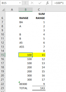
Result here (where cell B15 has a simple formula to demonstrate the criteria)
Conditionally Formatting if Cells Contain Errors
This can be useful to quickly highlight errors in your data.
To do this (or our range B7:C22) you can change your conditional format formula to:
=ISERROR(B7)
As we’ve taken out the absolute reference to column B (dollar sign $) this will check each cell individually in the range. ISERROR returns TRUE if cell B7 is an error.
One-Off Cell Attribute Tests
To avoid bogging your spreadsheet down with unnecessary conditional formatting, it is worth knowing how you can achieve similar results using GOTO SPECIAL CELLS.
Follow these steps to find and format cells with various attributes such as TEXT, FORMULA, BLANK, VISIBLE, ETC. In the example we’ll format any cell in our range that is TEXT.
We’ll keep using the same range but I’ve removed the conditional formats.
1. Start by highlighting the range.
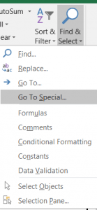
2. From the HOME RIBBON click FIND & SELECT -> GOTO SPECIAL…
3. From the following dialog select CONSTANTS then TEXT checkbox.
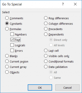
4. Click OK but don’t move the cursor once you’ve been returned to the spreadsheet
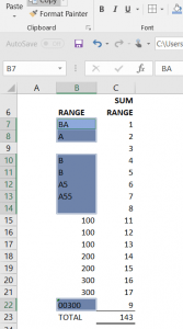
5. You will see that all the TEXT entries in your range are selected.
[Note if you are dealing with a large range you may want to change the zoom level by going to the VIEW RIBBON and selecting ZOOM TO SELECTION]
While these are selected you can format the cells. In the example I’ll go the HOME RIBBON and set the FILL to blue:
Conclusion
We’ve just scratched the surface with conditional formatting possibilities when using formulas. If you have any questions related to conditional formatting please post them in the comments below.

Leave a Comment