It can be incredibly useful to create a link to VLOOKUP results in Excel®. This is particularly true if you have used VLOOKUP to join data from one table to another. You can jump straight to the result of the VLOOKUP and see the rest of the data in that row of your Excel® table.
- We can quite easily create the join by using the HYPERLINK, ADDRESS and MATCH functions along with the VLOOKUP.
- Then with a slightly different solution we can make the formula more robust so it won’t be disrupted by changes to the worksheet name.
- An Excel® link to a dynamic SUMIF result
Excel® Link to VLOOKUP Result
This tutorial assumes you are familiar with the VLOOKUP function.
Note: our special links tools can create these links to VLOOKUP results in seconds.
HYPERLINK Function Background
The HYPERLINK function is less often used so lets start with that. HYPERLINK requires two arguments. The first is the LINK_LOCATION. I.e. the web address or in our case the file, sheet and cell address that Excel® will jump to when the link is clicked.
The link location can be a full file path such as
=HYPERLINK(“[C:\Users\Mike\Desktop\My Excel File.xlsx]’Sheet Name Here’!H6”,“CLICK LINK”)
Note the format of the LINK_LOCATION if you need to use the full path. The full location is in inverted commas “”. Within this the folder path and file name are contained in [] square brackets. The sheet name is within single inverted commas ‘. Then exclamation mark “!” is required prior to the cell reference.
The FRIENDLY_NAME can be any text you like.
Clearly if we are just linking to the current file it would be good if we could avoid the text for the path and filename. Particularly if there is a chance these could change. Thankfully Microsoft® provide a simple solution to this.
Replacing file path and name with ‘#’
The hash sign # can replace this full path and filename. So our Excel® link function above can be changed to:
=HYPERLINK(“#’LINK TO VLOOKUP RESULT’!H6”,“CLICK LINK”) – where our sheet name is “LINK TO VLOOKUP RESULT”
This is a lot tidier and more functional as a change to file path or name will not affect the function.
Now we’ve looked at the HYPERLINK function lets start our link to the VLOOKUP result.
Link to VLOOKUP Result
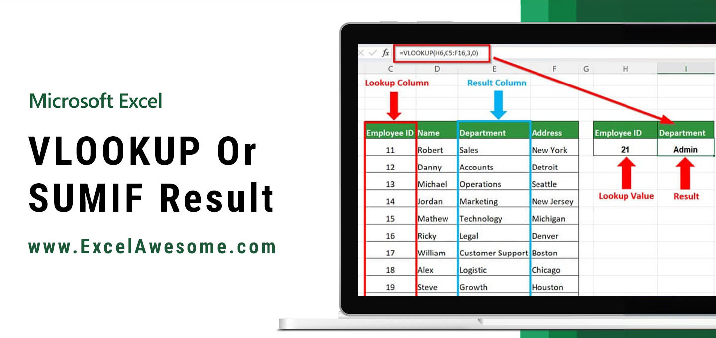
In the example we are going to work with this VLOOKUP as the basis for our link:
So this is returning our January figure for ‘Sales’.
Working out the cell ADDRESS to use for our Hyperlink function
The address used in our link to the result will need to be dynamic. I.e. when cell B11 changes from Operations to Sourcing the address will need to change from $C$20 to $C$22.
The ADDRESS function in Excel® requires the following arguments: ROW_NUM, COL_NUM. There are also the following optional arguments which we won’t need for now: ABS_NUM, A1, and SHEET NAME.
We’ll use cell C11 to develop our ADDRESS function for now.
The ROW_NUM calculation
To calculate the row number for the address we can do the following calculation: [the first row of our lookup table] + [the row in the table where we can find the VLOOKUP result].
[the first row of our lookup table]: ROW($C$17)
[the row in the table where we can find the VLOOKUP result]: MATCH($B11, $B$17:$B$27, 0)
The ROW formula will simply return 17 as being the start of our table.
The MATCH function will look down the first column of our table and return the number position of the matched item. For ‘Operations’ this will be 4.
The COL_NUM calculation
This one is easier in our example as we know the column should always be the second column in the lookup table (based on our VLOOKUP column selection). So simply using the following function will return the column number:
COLUMN($C$17)
So the ADDRESS function to get the cell with the VLOOKUP result is:
=ADDRESS(ROW($C$17) -1 + MATCH($B11, $B$17:$B$27, 0), COLUMN($C$17))
The HYPERLINK Function
Our final formula that will be our link to the vlookup result is as follows:
=HYPERLINK(“#” & ADDRESS(ROW($C$17) -1 + MATCH($B11, $B$17:$B$27, 0), COLUMN($C$17)), VLOOKUP($B11, $B$17:$O$27, 2, FALSE))
This will work whenever the lookup table is in the same sheet as our formula.
This can be easily adapted so we can copy it to a different sheet (it still needs to be in the same file).
Excel® link to VLOOKUP result for different sheet
To do this we just need to add the sheet reference to the ADDRESS and make sure that our references to the table include the sheet name (our sheet name is ‘LINK TO VLOOKUP RESULT’. So the ADDRESS function now looks like this:
=ADDRESS(ROW(‘LINK TO VLOOKUP RESULT’!$C$17) -1 + MATCH($B3, ‘LINK TO VLOOKUP RESULT’!$B$17:$B$27, 0), COLUMN(‘LINK TO VLOOKUP RESULT’!$C$17), , , “LINK TO VLOOKUP RESULT”)
Notice we can still ignore the other optional arguments in the ADDRESS function (hence the 3 commas together between the COL_NUM and the SHEET_NAME).
Putting this in to our HYPERLINK function we have:
=HYPERLINK(“#” & ADDRESS(ROW(‘LINK TO VLOOKUP RESULT’!$C$17) -1 + MATCH($B3, ‘LINK TO VLOOKUP RESULT’!$B$17:$B$27, 0), COLUMN(‘LINK TO VLOOKUP RESULT’!$C$17), , , “LINK TO VLOOKUP RESULT”), VLOOKUP($B3, ‘LINK TO VLOOKUP RESULT’!$B$17:$O$27, 2, FALSE))
This Excel® link to the VLOOKUP result should work really well for most occasions.
The limitation with this simple method:
We could run in to problems if the worksheet with the lookup table is renamed. As you can see in our formula, the sheet name has been hard-coded.
To Overcome This Limitation
We can overcome the sheet name problem by using the CELL function.
The CELL function can return various information about a particular cell. In our case we can use:
=CELL(“filename”, ‘LINK TO VLOOKUP RESULT’!$C$17).
This will return the full path, filename and sheet name: C:\Users\Mike\Desktop\[Excel Awesome Tutorials 20180323.xlsx]LINK TO VLOOKUP RESULT (where “LINK TO VLOOKUP RESULT” is the sheet name we want).
You can see from the result that we could use the string after the close square bracket ‘]’ to identify the sheet name.
The FIND function will be able to locate this for us:
=FIND(“]”, CELL(“filename”, ‘LINK TO VLOOKUP RESULT’!$C$17))
Finally we can use the MID function to just take the final characters. The MID function arguments are: TEXT, START_NUM, NUM_OF_CHARACTERS. The text will be our CELL function, start will be our FIND function and the number of characters just needs to be long enough to pick up any sheet name (it doesn’t matter if this number is larger than the remaining text). The maximum sheet name length in Excel® is 31 characters.
So our final formula to get the sheet name is:
=MID(CELL(“filename”, ‘LINK TO VLOOKUP RESULT’!$C$17), FIND(“]”, CELL(“filename”, ‘LINK TO VLOOKUP RESULT’!$C$17))+1, 31)
Finalizing the Excel® Link to VLOOKUP Results
We can now go back to our HYPERLINK formula. Within that formula, locate the sheet name in the ADDRESS function. Now replace the hard-coded sheet name with the MID function we’ve just developed (see Fig(a6) below).
Our final formula is:
=HYPERLINK(“#” & ADDRESS(ROW(‘LINK TO VLOOKUP RESULT’!$C$17) -1 + MATCH($B11, ‘LINK TO VLOOKUP RESULT’!$B$17:$B$27, 0), COLUMN(‘LINK TO VLOOKUP RESULT’!$C$17), , , MID(CELL(“filename”, ‘LINK TO VLOOKUP RESULT’!$C$17), FIND(“]”, CELL(“filename”, ‘LINK TO VLOOKUP RESULT’!$C$17))+1, 31)), VLOOKUP($B11, ‘LINK TO VLOOKUP RESULT’!$B$17:$O$27, 2, FALSE))
If you want to go on to look at a similar exercise then the last part of this tutorial looks at links to SUMIF results.
Excel® Link to Dynamic SUMIF Result
We can use similar functionality with SUMIF formulas. This is going to take things a step further. But this is probably even more useful as we’re going to be able to jump to a whole range of data that meets the SUMIF criteria. This does require the SUMIF criteria range to be sorted.
We’re going to have a dynamic SUMIF function in this example. This looks in the appropriate month column in our table. So if we select ‘1’ we get January results; if we select ‘2’ we get February results and so on.
Before we look at the link lets first consider how we can build the dynamic function with SUMIF.
Our Dynamic SUMIF Function
Lets start by reviewing the SUMIF function used in the case. SUMIF arguments are: CRITERIA_RANGE, CRITERIA and SUM_RANGE.
Our criteria range is $B$13:$B$36. In here we’re looking for the value in cell B11.
Our sum range is the dynamic part of the SUMIF: we’re going to set the column to sum from our table based on the entry in cell C11.
OFFSET To Shift Our SUMIF Sum Range
This dynamic function is achieved by using the OFFSET function. OFFSET arguments are REFERENCE, ROWS, COLUMNS, [HEIGHT] and [WIDTH]. We don’t need to worry about the final two optional arguments on this occasion.
Our reference is the same as the SUMIF criteria range (B13:B36). We’re going to use this as the basis for our for our dynamic range.
The rows number will shift our reference range either up or down based on this value. We won’t be moving the rows of the range so our ROWS value will be zero.
Columns shifts the reference range right or left based on this value. We want to shift our reference range right based on the entry in cell C11. The number of columns to shift right can be determined by finding cell C11 in the headings in range C13:N13. This can be identified by the following formula:
MATCH($C$11, $C$13:$N$13, 0)
Putting the reference, rows and columns in to our OFFSET function looks like this:
= OFFSET( $B$13:$B$36, 0, MATCH($C$11, $C$13:$N$13, 0))
You can see the final SUMIF below:
=SUMIF( $B$13:$B$36, $B$11, OFFSET( $B$13:$B$36, 0, MATCH($C$11, $C$13:$N$13, 0)) )
Now we have our dynamic SUMIF function we can start to develop the link to result function.
ADDRESS For Link to SUMIF Result
As the formula is even longer in this instance we’ve kept the filename, sheet name and address functions separate in cells C6:C8.
The filename and sheet names are identified in the same way as the link to VLOOKUP result earlier in this page.
The address is slightly more complicated as we have to identify the top left cell and the bottom right cell of the range in the HYPERLINK.
As you can see in the image below, the formula in cell C8 is shown in cell I8 for information. There are 2 address functions for top left and bottom right joined by “:”.
Top left address
The first top left ADDRESS row number for B13 plus the row where we find the value in B11 (identified by a MATCH function):
=ROW($B$13) + MATCH($B$11, $B$14:$B$36, 0)
The column is identified in a similar manner. This time the MATCH function looks along the column headings C13:N13:
=COLUMN($B$13) + MATCH($C$11, $C$13:$N$13, 0 )
Bottom right address
The bottom of the range defined by the second ADDRESS is almost identical. The only difference is the need to find the last row of cells that matches the ‘Item’ criteria. To do this we need to use a COUNTIF of the matched ‘Items’ to add to the row calculation:
=ROW($B$13) + MATCH($B$11, $B$14:$B$36, 0) + COUNTIF($B$14:$B$36, $B$11) -1
Complete address for use in our link
Putting that altogether we have the following full address formula to use in our hyperlink to the SUMIF result:
=ADDRESS(ROW($B$13) + MATCH($B$11, $B$14:$B$36, 0), COLUMN($B$13) + MATCH($C$11, $C$13:$N$13, 0 )) & “:” &ADDRESS(ROW($B$13) + MATCH($B$11, $B$14:$B$36, 0) + COUNTIF($B$14:$B$36, $B$11) -1, COLUMN($B$13) + MATCH($C$11, $C$13:$N$13, 0 ))
The Final Excel® Link to SUMIF Result
We now have all the components needed for the final formula. The link address is now in cells C6:C8. We just need to join these as the HYPERLINK LOCATION_ADDRESS and use the dynamic SUMIF calculation as the FRIENDLY_NAME.
=HYPERLINK(C6 & C7 & C8, SUMIF( $B$13:$B$36, $B$11, OFFSET( $B$13:$B$36, 0, MATCH($C$11, $C$13:$N$13, 0))))
Conclusion
There is a little work to put this together the first time. But the result will be worth it when you (or your spreadsheet users) need to drill down to details.
Learn more about VLOOKUP: Lookup Part of Text in a Cell.
Leave a Comment